In the Department of Biochemistry and Structural Biology at UT Health San Antonio, we work at the interface between molecular structures and cell, tissue, and organ function to probe the essential molecular mechanisms of life and disease. Research in the labs of our faculty spans many disciplines, including:
UT Health San Antonio Department of Biochemistry and Structural Biology
We work at the interface between molecular structures and cell, tissue, and organ function to probe the essential molecular mechanisms of life and disease and design novel therapies
- Cancer Biochemistry/genomic integrity
- Neurobiological Mechanisms
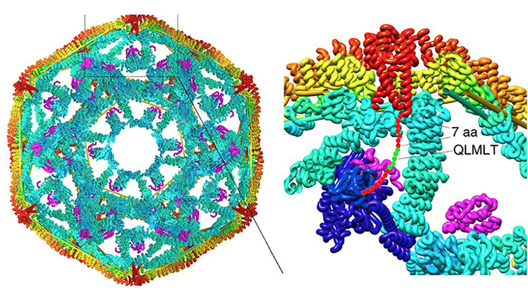
- Parasite/Viral Mechanisms
- Computational Biology, Bioinformatics
- Enzymology/Metabolic Regulation
- Proteomics and Metabolomics
- Structural Biology
- Intercellular Signaling pathways
One hallmark of our program is a focus on developing the next generation of therapeutics targeting cancer, infectious diseases and neuronal regeneration. Our faculty have made seminal contributions to many of these areas, and include Fellows of the American Association for the Advancement of Science, past-presidents of three national societies and 5 Presidential Distinguished Research and Teaching Faculty. Our graduate students are also a diverse group representing 4 disciplines within the IBMS (The department is the primary host for the Biochemical Mechanisms in Disease , MD/PhD and Biomedical engineering students and visiting foreign students from several programs.
The technically complex nature of the molecular and biophysical studies conducted within the Department demands sophisticated instrumentation which is housed in several core facilities, each of which operates under the guidance of an internationally recognized expert:
- Macromolecular Interactions – Calorimetry (ITC, DSC), Surface Plasmon Resonance (SPR), Light Scattering (DLS, SLS), AUC , and PEPcore
- Mass Spectrometry – Proteomics/Metabolomics
- High Throughput Screening for Drug Discovery
- NMR Spectroscopy/Fragment-based Screening
- X-ray Crystallography
On behalf of the faculty, students, researchers and staff in the Department, I invite you to get in touch with us — we will be happy to visit with you. Our contact information can be found in the People and the Department Contacts sections on this webpage.
Biochemistry and Structural Biology
7703 Floyd Curl Dr.
4th Floor, Mail Code 7760
San Antonio, TX 78229-3900
Voice: (210) 567-3770
Fax: (210) 567-6595